Machine Learning — Lecture Notes A complete beginner-friendly guide covering theory, mathematics, kernel methods, and real-world applications
Table of Contents
- Linear Classifiers
- Classifier Margin
- Maximum Margin & Linear SVM
- SVM Mathematics
- Solving the Optimization Problem
- Noisy Data & Soft Margin Classification
- Non-linear SVMs & the Kernel Trick
- Properties of SVM
- Real-World Applications
- Limitations of SVM
Linear Classifiers
A classifier is a function that takes a data point and assigns it to one of several predefined classes. In the binary case, we have two classes — conventionally labeled +1 and −1.
A linear classifier separates these classes using a straight line (in 2D), a plane (in 3D), or more generally a hyperplane in higher-dimensional space.
Core Formula
- — the weight vector, which is perpendicular to the decision boundary and controls its orientation
- — the input feature vector (your data point)
- — the bias (also called intercept), which shifts the boundary away from the origin
- The output is +1 or −1 depending on which side of the hyperplane the point falls
How the Decision Rule Works
The expression computes a score for each input:
- Score > 0 → classify as +1 (positive class)
- Score < 0 → classify as −1 (negative class)
- Score = 0 → the point lies exactly on the decision boundary
The Fundamental Problem: Infinitely Many Valid Boundaries
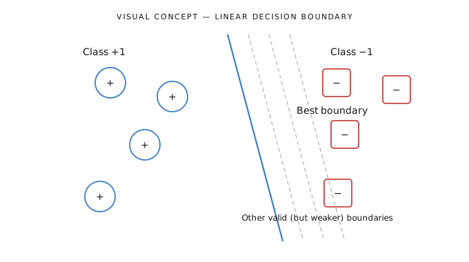
When two classes are perfectly separable, there exist infinitely many hyperplanes that correctly separate them. Each gives zero training error, but they will generalize differently on unseen data. This raises the key question:
Which hyperplane should we choose?
This is precisely the problem Support Vector Machines are designed to solve.
Classifier Margin
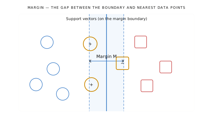
The margin is the distance between the decision boundary and the nearest data points from either class. These nearest points are called support vectors (introduced formally in the next section).
Intuitive Analogy
Think of building a road between two rows of houses. The margin is the road's total width. A wider road is safer — vehicles (new data points) have more room before hitting a house (being misclassified). You want to build the widest road possible.
Why a Larger Margin Generalizes Better
A boundary with a large margin is more robust to perturbations. If new data arrives slightly displaced from the training data, a large-margin classifier is less likely to misclassify it. This is formally justified by PAC (Probably Approximately Correct) learning theory, which proves:
In other words, maximizing the margin directly minimizes an upper bound on future classification error.
Maximum Margin & Linear SVM
The Support Vector Machine finds the unique hyperplane that maximizes the margin between the two classes. This is also called the Maximum Margin Classifier or Linear SVM (LSVM).
★ Key Insight
The data points lying exactly on the margin boundaries are the support vectors. They are the only points that define the optimal hyperplane. All other training points are irrelevant — you could remove them without changing the result.
| Property | Explanation |
|---|---|
| Maximizing margin is principled | Both geometric intuition and PAC learning theory confirm that a larger margin improves generalization. |
| Only support vectors matter | After training, the classifier depends only on support vectors. Other points have no influence on the boundary. |
| Strong empirical performance | SVM consistently achieves excellent results, especially on high-dimensional data. |
SVM Mathematics
Defining the Three Key Hyperplanes
We define three parallel hyperplanes that characterize the SVM solution:
Decision boundary (the central separating hyperplane):
Positive margin boundary (touches positive support vectors):
Negative margin boundary (touches negative support vectors):
The constraints require that no training point falls between these two margin boundaries:
Computing the Margin Width
Step 1 — Pick one point from each boundary.
Let be a support vector on and be a support vector on . By definition:
Step 2 — Subtract to relate the two points.
Step 3 — Project onto the normal direction .
The vector points from to but is not necessarily perpendicular to the boundaries. The perpendicular distance (the margin ) is obtained by projecting onto the unit normal :
Step 4 — Substitute the result from Step 2.
Optimization Objective
To maximize the margin , we minimize . For convenience, we minimize the squared norm:
subject to:
This is a convex quadratic program with linear constraints — it has a unique global minimum and can be solved efficiently.
Solving the Optimization Problem
Why Use Lagrange Multipliers?
The SVM optimization has linear constraints, making it ideal for the Lagrangian method. Rather than solving the constrained problem directly, we transform it into an unconstrained dual problem that is often easier to solve and reveals important structure.
Step 1 — Form the Lagrangian
Introduce a non-negative multiplier for each training constraint:
At the optimum, increasing any for a non-binding constraint does not help, so the Lagrangian captures all the information in the original problem.
Step 2 — Derive Stationarity Conditions
Setting the partial derivatives to zero:
Important: The weight vector is a linear combination of the training points, weighted by their values. Points with contribute nothing — these are the non-support vectors.
Step 3 — The Dual Problem
Substituting the stationarity conditions back into the Lagrangian eliminates and , yielding the dual problem:
Subject to:
Key Observations
1. Sparsity: After solving, most . Only the support vectors have . This means the classifier stores and uses only a small subset of training data.
2. Data appears only as dot products : This is the critical structural property that enables the kernel trick (Section 07). We can replace dot products with any valid kernel without changing the optimization procedure.
Making Predictions
Once is found, the bias is recovered from any support vector:
The classifier for a new point is:
Noisy Data & Soft Margin Classification
The Problem with Hard Margin SVM
The formulation above assumes data is perfectly linearly separable — no overlap, no noise, no outliers. In practice:
- Real-world data almost always has noise and mislabeled examples
- Forcing zero training error on noisy data causes overfitting: the boundary contorts to accommodate every outlier and performs poorly on new data
- For slightly non-separable data, the hard margin problem is infeasible (no solution exists)
Solution: Slack Variables (Soft Margin SVM)
We introduce slack variables , one per training point, that allow controlled violation of the margin constraints.
Interpretation of :
| Value | Meaning |
|---|---|
| Point is correctly classified and outside the margin — no violation | |
| Point is correctly classified but falls inside the margin | |
| Point is misclassified |
The Soft Margin Optimization Problem
Subject to:
The objective has two competing terms:
- — maximize the margin
- — minimize total margin violations
The Role of the Regularization Parameter C
| C Value | Effect | Risk |
|---|---|---|
| Large | Penalizes violations heavily; tries to classify all training points correctly | Overfitting to noise |
| Small | Tolerates more violations in exchange for a wider margin | Underfitting if C is too small |
In practice, is chosen using cross-validation.
Hard vs. Soft Margin Comparison
| Hard Margin SVM | Soft Margin SVM |
|---|---|
| Requires perfectly separable data | Handles overlapping, noisy data |
| Infeasible if data overlaps | Always has a solution |
| Zero training misclassifications | Allows controlled misclassifications |
| Constraint: | Constraint: |
| No tuning parameter | Tuning parameter controls bias-variance trade-off |
Non-linear SVMs & the Kernel Trick
When Linear Boundaries Are Insufficient
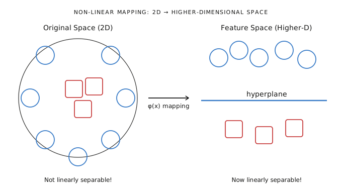
Some datasets cannot be separated by any hyperplane. Consider a ring of red points surrounded by blue points — no straight line separates them. A linear SVM will fail here regardless of the margin.
The Core Idea: Feature Space Mapping
The key insight is to map the data into a higher-dimensional feature space using a function , where the classes become linearly separable. We then apply a linear SVM in this higher-dimensional space.
Example
Consider 2D data lying on concentric circles (not linearly separable). Add a third feature . In 3D space, the inner circle has small values and the outer circle has large values — they are now separated by the plane . This plane corresponds to a circle in the original 2D space.
The Computational Problem — and Its Elegant Solution
Explicitly computing for a very high (or infinite) dimensional space is prohibitively expensive. However, notice that in the SVM dual problem, data only appears as dot products . After mapping, these become .
A kernel function computes this dot product directly in the original space, without ever computing explicitly:
This is the kernel trick: replace every dot product with a kernel evaluation, and the SVM works implicitly in a potentially infinite-dimensional space at the cost of computing kernel values.
Worked Example — Polynomial Kernel
For 2D vectors , the kernel implicitly corresponds to the 6-dimensional mapping:
The kernel computes the 6D dot product using only 2D arithmetic — a significant computational saving.
What Makes a Valid Kernel? (Mercer's Theorem)
A function is a valid kernel if and only if the Gram matrix with entries is symmetric and positive semi-definite for any set of inputs. You do not need to explicitly construct — just verify this condition.
Common Kernel Functions
| Kernel | Formula | Best Used When |
|---|---|---|
| Linear | Data is already linearly separable; very high-dimensional (e.g., text) | |
| Polynomial (degree ) | Text classification; polynomial decision boundaries | |
| Gaussian / RBF | General-purpose default; smooth, locally varying boundaries | |
| Sigmoid | Resembles neural network activation; only valid for certain parameters |
The Non-linear SVM Dual Problem
Replacing dot products with kernel evaluations in the dual:
The decision function becomes:
The optimization algorithm is identical to the linear case — only the inner products are replaced by kernel evaluations.
Properties of SVM
| Property | Description |
|---|---|
| Flexible similarity measure | The kernel function defines what "similar" means. You can design custom kernels for strings, graphs, images, or any structured data. |
| Sparse solution | Only support vectors () are stored and used at prediction time. For large datasets, this can be a tiny fraction of the training data. |
| Handles high-dimensional data | Generalization bounds depend on the margin, not the number of features. SVM does not degrade as dimensionality increases — unlike many other classifiers. |
| Overfitting control | The regularization parameter in soft-margin SVM provides a direct, principled mechanism to balance fitting the training data and generalizing to new data. |
| Guaranteed global optimum | The primal objective is convex and the constraints are linear. The optimization has exactly one global minimum — no local minima exist. |
| Implicit feature selection | In the linear SVM, the squared weight quantifies the contribution of feature . Features with small weights can be pruned without significant performance loss. |
Real-World Applications
Application 1 — Cancer Classification via Gene Expression Data
The Challenge
| Challenge | Details |
|---|---|
| High dimensionality () | Thousands of gene expression measurements per patient, but typically fewer than 100 patients. Standard methods break down in this regime. |
| Class imbalance | Far fewer cancer-positive than cancer-negative samples. Naive classifiers are biased toward the majority class. |
| Noisy, irrelevant features | Most genes are unrelated to the cancer subtype being classified. They contribute noise that can mislead other classifiers. |
How SVM Addresses Each Challenge
Handling imbalance: A modified kernel adds a correction term proportional to the fraction of positive samples:
where is the number of positive training examples and is the total. This re-balances the effective cost of misclassifying minority-class examples.
Feature selection: In the linear SVM, the weight magnitude ranks each gene by importance. Genes with very small weights are likely irrelevant and can be removed — a process called recursive feature elimination (RFE).
High-dimensional stability: SVM's generalization bound depends on the margin, not the number of features. This makes it particularly well-suited to the regime of genomic data.
Known Limitation
SVM is sensitive to label noise (mislabeled training examples). Even a small fraction of incorrectly labeled patients can significantly degrade classification performance. Careful data curation is essential.
Application 2 — Text Categorization
The Task
Automatically assign text documents (news articles, emails, web pages) to predefined categories. Since a document can belong to multiple categories, this is decomposed into a set of independent binary classification problems — one per category (e.g., "politics vs. not politics", "sports vs. not sports").
Representing Documents as Vectors: Bag of Words (TF-IDF)
Before SVM can process text, documents must be converted to numerical vectors:
- Build a vocabulary of all words appearing in the training corpus (after preprocessing).
- Preprocess: Remove stop words ("the", "is", "a") and apply stemming (map "running", "runs", "ran" → "run").
- Assign TF-IDF weights to each word per document:
where is the term frequency (how often word appears in the document), is the inverse document frequency ( = number of documents containing word , = total documents), and is a normalization constant. This down-weights common words and up-weights discriminative words.
- The result is a sparse, high-dimensional vector where most entries are zero (most words don't appear in any given document).
Why SVM Is a Natural Fit for Text
| Reason | Explanation |
|---|---|
| Very high dimensionality | Vocabularies of 50,000–100,000 words are common. SVM handles this natively; many other classifiers cannot. |
| Sparse instances | Each document uses only a tiny fraction of all vocabulary words. SVM's sparse support vector structure aligns perfectly with this. |
| Dense concept structure | Unlike gene data, most words are relevant to at least some categories. There are few truly irrelevant features. |
| Empirical linear separability | Text categorization problems have been found to be approximately linearly separable in high-dimensional word space. Linear SVM is therefore both fast and effective. |
Limitations of SVM
Limitations 1 — Sensitivity to Label Noise
Mislabeled training examples can have a disproportionate effect on the decision boundary (particularly if they become support vectors). This is especially problematic in medical applications where annotation errors are common.
Limitations 2 — Inherently Binary
Standard SVM is formulated for two-class problems. Real tasks often require distinguishing among classes.
Extending SVM to Multi-class Problems
The standard approach is one-vs-rest (OvR) classification:
- Train separate SVMs. SVM- is trained to distinguish class from all other classes (positive label = class , negative label = all others).
- To classify a new point , evaluate all classifiers.
- Assign the class whose classifier gives the largest positive score (i.e., the point is furthest into the positive region):
Practical Guidelines for Applying SVM
| Decision | Recommendation |
|---|---|
| Kernel selection | Start with the RBF (Gaussian) kernel as a default. Use a linear kernel for very high-dimensional data (text, genomics). Design custom kernels for structured inputs (graphs, sequences). |
| Setting in RBF kernel | Initialize to the average or median pairwise distance between training points of different classes. Tune further with cross-validation. |
| Setting (regularization) | Use -fold cross-validation or a held-out validation set. There is no universal optimal value — it depends on the noise level and overlap in your data. |
★ Summary
SVM remains one of the most theoretically well-grounded classifiers in machine learning. Its convex optimization guarantees a unique global solution. The kernel trick provides principled non-linear generalization at manageable computational cost. The soft margin formulation handles real-world noise robustly. Despite the rise of deep learning, SVM continues to be competitive — and often superior — on small, high-dimensional datasets such as those encountered in genomics, text analysis, and medical diagnostics.