Table of Contents
What is PCA? When to Use PCA Mathematical Foundations General Rules and Key Formulas Step-by-Step Algorithm Numerical Example 1 — 2 Features (Math & Physics) Numerical Example 2 — 3 Features (Student Exam Scores) Geometric Intuition Explained Variance Choosing the Number of Components Limitations of PCA Summary
What is PCA?
Principal Component Analysis (PCA) is a linear dimensionality reduction technique that transforms a dataset with possibly correlated variables into a new coordinate system where the axes (called principal components ) are ordered by the amount of variance they capture from the original data.
PCA finds the directions of maximum variance in high-dimensional data and projects it onto a lower-dimensional subspace while retaining as much information as possible.
Core Idea
Given a dataset with
n
n
n
p
p
p
p
p
p
Orthogonal (uncorrelated with each other)Ordered by the amount of variance they explainLinear combinations of the original features
When to Use PCA
Situation
Use PCA?
High-dimensional data (
p
≫
n
p \gg n
p ≫ n
✅ Yes
Multicollinearity among features
✅ Yes
Need for 2D/3D visualization
✅ Yes
Features are on different scales
✅ Yes (after standardization)
Non-linear relationships in data
❌ No (use Kernel PCA)
Need interpretable features
❌ No (PCA components are abstract)
Categorical features
❌ No (use MCA instead)
Mathematical Foundations
Vectors and Matrices
A dataset of
n
n
n
p
p
p
X
=
[
x
11
x
12
⋯
x
1
p
x
21
x
22
⋯
x
2
p
⋮
⋮
⋱
⋮
x
n
1
x
n
2
⋯
x
n
p
]
∈
R
n
×
p
X = \begin{bmatrix} x_{11} & x_{12} & \cdots & x_{1p} \\ x_{21} & x_{22} & \cdots & x_{2p} \\ \vdots & \vdots & \ddots & \vdots \\ x_{n1} & x_{n2} & \cdots & x_{np} \end{bmatrix} \in \mathbb{R}^{n \times p}
X =
x 11 x 21 ⋮ x n 1 x 12 x 22 ⋮ x n 2 ⋯ ⋯ ⋱ ⋯ x 1 p x 2 p ⋮ x n p
∈ R n × p Mean Vector
x
ˉ
=
1
n
∑
i
=
1
n
x
i
=
[
x
ˉ
1
x
ˉ
2
⋮
x
ˉ
p
]
\bar{\mathbf{x}} = \frac{1}{n} \sum_{i=1}^{n} \mathbf{x}_i = \begin{bmatrix} \bar{x}_1 \\ \bar{x}_2 \\ \vdots \\ \bar{x}_p \end{bmatrix}
x ˉ = n 1 i = 1 ∑ n x i =
x ˉ 1 x ˉ 2 ⋮ x ˉ p
Variance
Var
(
X
j
)
=
σ
j
2
=
1
n
−
1
∑
i
=
1
n
(
x
i
j
−
x
ˉ
j
)
2
\text{Var}(X_j) = \sigma_j^2 = \frac{1}{n-1} \sum_{i=1}^{n} (x_{ij} - \bar{x}_j)^2
Var ( X j ) = σ j 2 = n − 1 1 i = 1 ∑ n ( x ij − x ˉ j ) 2 Covariance
Cov
(
X
j
,
X
k
)
=
σ
j
k
=
1
n
−
1
∑
i
=
1
n
(
x
i
j
−
x
ˉ
j
)
(
x
i
k
−
x
ˉ
k
)
\text{Cov}(X_j, X_k) = \sigma_{jk} = \frac{1}{n-1} \sum_{i=1}^{n} (x_{ij} - \bar{x}_j)(x_{ik} - \bar{x}_k)
Cov ( X j , X k ) = σ j k = n − 1 1 i = 1 ∑ n ( x ij − x ˉ j ) ( x ik − x ˉ k )
Note:
Cov
(
X
j
,
X
j
)
=
Var
(
X
j
)
\text{Cov}(X_j, X_j) = \text{Var}(X_j)
Cov ( X j , X j ) = Var ( X j )
Cov
(
X
j
,
X
k
)
=
Cov
(
X
k
,
X
j
)
\text{Cov}(X_j, X_k) = \text{Cov}(X_k, X_j)
Cov ( X j , X k ) = Cov ( X k , X j )
Covariance Matrix
Σ
=
[
σ
1
2
σ
12
⋯
σ
1
p
σ
21
σ
2
2
⋯
σ
2
p
⋮
⋮
⋱
⋮
σ
p
1
σ
p
2
⋯
σ
p
2
]
\Sigma = \begin{bmatrix} \sigma_1^2 & \sigma_{12} & \cdots & \sigma_{1p} \\ \sigma_{21} & \sigma_2^2 & \cdots & \sigma_{2p} \\ \vdots & \vdots & \ddots & \vdots \\ \sigma_{p1} & \sigma_{p2} & \cdots & \sigma_p^2 \end{bmatrix}
Σ =
σ 1 2 σ 21 ⋮ σ p 1 σ 12 σ 2 2 ⋮ σ p 2 ⋯ ⋯ ⋱ ⋯ σ 1 p σ 2 p ⋮ σ p 2
In matrix form, using the centered data matrix
X
′
X'
X ′
X
′
=
X
−
X
ˉ
X' = X - \bar{X}
X ′ = X − X ˉ
Σ
=
1
n
−
1
X
′
T
X
′
\boxed{\Sigma = \frac{1}{n-1} X'^T X'}
Σ = n − 1 1 X ′ T X ′
z
i
j
=
x
i
j
−
x
ˉ
j
σ
j
z_{ij} = \frac{x_{ij} - \bar{x}_j}{\sigma_j}
z ij = σ j x ij − x ˉ j
General Rule: Always standardize when features are measured on different scales. Skip standardization only when features are already on the same scale.
Σ
v
=
λ
v
⟺
det
(
Σ
−
λ
I
)
=
0
\Sigma \mathbf{v} = \lambda \mathbf{v} \quad \Longleftrightarrow \quad \boxed{\det(\Sigma - \lambda I) = 0}
Σ v = λ v ⟺ det ( Σ − λ I ) = 0 Key properties of eigenvalues:
All eigenvalues are real and non-negative (
λ
≥
0
\lambda \geq 0
λ ≥ 0
∑
i
=
1
p
λ
i
=
trace
(
Σ
)
\sum_{i=1}^{p} \lambda_i = \text{trace}(\Sigma)
∑ i = 1 p λ i = trace ( Σ )
Key properties of eigenvectors:
Eigenvectors for distinct eigenvalues are orthogonal
Each eigenvector is a unit vector:
∥
v
i
∥
=
1
\|\mathbf{v}_i\| = 1
∥ v i ∥ = 1
Explained Variance Ratio
i
=
λ
i
∑
j
=
1
p
λ
j
\boxed{\text{Explained Variance Ratio}_i = \frac{\lambda_i}{\sum_{j=1}^{p} \lambda_j}}
Explained Variance Ratio i = ∑ j = 1 p λ j λ i
95% Rule: Select minimum
k
k
k
∑
i
=
1
k
λ
i
∑
j
=
1
p
λ
j
≥
0.95
\dfrac{\sum_{i=1}^{k} \lambda_i}{\sum_{j=1}^{p} \lambda_j} \geq 0.95
∑ j = 1 p λ j ∑ i = 1 k λ i ≥ 0.95
Z
=
X
′
W
k
\boxed{Z = X' W_k}
Z = X ′ W k where
X
′
∈
R
n
×
p
X' \in \mathbb{R}^{n \times p}
X ′ ∈ R n × p
W
k
∈
R
p
×
k
W_k \in \mathbb{R}^{p \times k}
W k ∈ R p × k
k
k
k
Z
∈
R
n
×
k
Z \in \mathbb{R}^{n \times k}
Z ∈ R n × k
X
^
=
Z
W
k
T
+
X
ˉ
Reconstruction Error
=
∑
i
=
k
+
1
p
λ
i
\hat{X} = Z W_k^T + \bar{X} \qquad \text{Reconstruction Error} = \sum_{i=k+1}^{p} \lambda_i
X ^ = Z W k T + X ˉ Reconstruction Error = i = k + 1 ∑ p λ i Rule 6: Correlation vs. Covariance PCA
Covariance PCA
Correlation PCA
Input
Mean-centered data
Standardized data (
z
z
z
Matrix used
1
n
−
1
X
′
T
X
′
\frac{1}{n-1}X'^TX'
n − 1 1 X ′ T X ′ Correlation matrix
R
R
R
When to use
Same units/scale
Different units/scale
Rule 7: Loadings vs. Scores
Term
Symbol
Meaning
Formula
Loadings
W
W
W Eigenvectors; direction of PCs in original space
Σ
W
=
W
Λ
\Sigma W = W \Lambda
Σ W = W Λ
Scores
Z
Z
Z Projected data in PC space
Z
=
X
′
W
Z = X'W
Z = X ′ W
Eigenvalue
λ
i
\lambda_i
λ i Variance of
i
i
i
Var
(
Z
i
)
=
λ
i
\text{Var}(Z_i) = \lambda_i
Var ( Z i ) = λ i
Step-by-Step Algorithm
Algorithm: Principal Component Analysis (PCA)
Input: Data matrix X ∈ ℝⁿˣᵖ, number of components k Output: Projected data Z ∈ ℝⁿˣᵏ, eigenvectors W, eigenvalues λ
Step 1: STANDARDIZE (if needed) For each feature j: x'ᵢⱼ = (xᵢⱼ - x̄ⱼ) / σⱼ
Step 2: CENTER THE DATA x̄ = (1/n) Σᵢ xᵢ X' = X - x̄ (subtract mean from each row)
Step 3: COMPUTE COVARIANCE MATRIX Σ = (1/(n-1)) X'ᵀ X'
Step 4: EIGENDECOMPOSITION Solve: det(Σ - λI) = 0 → find λ₁ ≥ λ₂ ≥ ... ≥ λₚ For each λᵢ: solve (Σ - λᵢI)vᵢ = 0 → find unit eigenvector vᵢ
Step 5: SORT BY EIGENVALUE (descending) Sort pairs (λ₁, v₁), (λ₂, v₂), ..., (λₚ, vₚ)
Step 6: SELECT TOP-k COMPONENTS W_k = [v₁ | v₂ | ... | vₖ] ∈ ℝᵖˣᵏ
Step 7: PROJECT DATA Z = X' · W_k ∈ ℝⁿˣᵏ
Numerical Example 1 — 2 Features (Math & Physics)
Scope:
n
=
5
n = 5
n = 5
p
=
2
p = 2
p = 2
k
=
1
k = 1
k = 1 (See PCA_Charts.html — Example 1 tab for the Scree Plot and PC1 Score chart.)
Step 1 — Collect the Data
Student
X
1
X_1
X 1
X
2
X_2
X 2
Student 1
85
80
Student 2
90
88
Student 3
70
65
Student 4
95
92
Student 5
60
58
Step 2 — Compute the Mean
X
ˉ
1
=
85
+
90
+
70
+
95
+
60
5
=
400
5
=
80
\bar{X}_1 = \frac{85 + 90 + 70 + 95 + 60}{5} = \frac{400}{5} = 80
X ˉ 1 = 5 85 + 90 + 70 + 95 + 60 = 5 400 = 80
X
ˉ
2
=
80
+
88
+
65
+
92
+
58
5
=
383
5
=
76.6
\bar{X}_2 = \frac{80 + 88 + 65 + 92 + 58}{5} = \frac{383}{5} = 76.6
X ˉ 2 = 5 80 + 88 + 65 + 92 + 58 = 5 383 = 76.6
x
ˉ
=
[
80
76.6
]
\bar{\mathbf{x}} = \begin{bmatrix} 80 \\ 76.6 \end{bmatrix}
x ˉ = [ 80 76.6 ] Step 3 — Center the Data
X
′
=
X
−
x
ˉ
T
=
[
85
−
80
80
−
76.6
90
−
80
88
−
76.6
70
−
80
65
−
76.6
95
−
80
92
−
76.6
60
−
80
58
−
76.6
]
=
[
5
3.4
10
11.4
−
10
−
11.6
15
15.4
−
20
−
18.6
]
X' = X - \bar{\mathbf{x}}^T =
\begin{bmatrix}
85-80 & 80-76.6 \\
90-80 & 88-76.6 \\
70-80 & 65-76.6 \\
95-80 & 92-76.6 \\
60-80 & 58-76.6
\end{bmatrix}
=
\begin{bmatrix}
5 & 3.4 \\
10 & 11.4 \\
-10 & -11.6 \\
15 & 15.4 \\
-20 & -18.6
\end{bmatrix}
X ′ = X − x ˉ T =
85 − 80 90 − 80 70 − 80 95 − 80 60 − 80 80 − 76.6 88 − 76.6 65 − 76.6 92 − 76.6 58 − 76.6
=
5 10 − 10 15 − 20 3.4 11.4 − 11.6 15.4 − 18.6
Step 4 — Compute the Covariance Matrix
Σ
=
1
N
−
1
X
′
T
X
′
=
1
4
X
′
T
X
′
\Sigma = \frac{1}{N-1}\,X'^T X' = \frac{1}{4}\,X'^T X'
Σ = N − 1 1 X ′ T X ′ = 4 1 X ′ T X ′
Cov
(
X
1
,
X
1
)
=
5
2
+
10
2
+
(
−
10
)
2
+
15
2
+
(
−
20
)
2
4
=
25
+
100
+
100
+
225
+
400
4
=
850
4
=
212.5
\text{Cov}(X_1,X_1) = \frac{5^2+10^2+(-10)^2+15^2+(-20)^2}{4}
= \frac{25+100+100+225+400}{4} = \frac{850}{4} = 212.5
Cov ( X 1 , X 1 ) = 4 5 2 + 1 0 2 + ( − 10 ) 2 + 1 5 2 + ( − 20 ) 2 = 4 25 + 100 + 100 + 225 + 400 = 4 850 = 212.5
Cov
(
X
2
,
X
2
)
=
3.4
2
+
11.4
2
+
(
−
11.6
)
2
+
15.4
2
+
(
−
18.6
)
2
4
=
11.56
+
129.96
+
134.56
+
237.16
+
345.96
4
=
859.2
4
=
214.8
\text{Cov}(X_2,X_2) = \frac{3.4^2+11.4^2+(-11.6)^2+15.4^2+(-18.6)^2}{4}
= \frac{11.56+129.96+134.56+237.16+345.96}{4} = \frac{859.2}{4} = 214.8
Cov ( X 2 , X 2 ) = 4 3. 4 2 + 11. 4 2 + ( − 11.6 ) 2 + 15. 4 2 + ( − 18.6 ) 2 = 4 11.56 + 129.96 + 134.56 + 237.16 + 345.96 = 4 859.2 = 214.8
Cov
(
X
1
,
X
2
)
=
(
5
)
(
3.4
)
+
(
10
)
(
11.4
)
+
(
−
10
)
(
−
11.6
)
+
(
15
)
(
15.4
)
+
(
−
20
)
(
−
18.6
)
4
\text{Cov}(X_1,X_2) = \frac{(5)(3.4)+(10)(11.4)+(-10)(-11.6)+(15)(15.4)+(-20)(-18.6)}{4}
Cov ( X 1 , X 2 ) = 4 ( 5 ) ( 3.4 ) + ( 10 ) ( 11.4 ) + ( − 10 ) ( − 11.6 ) + ( 15 ) ( 15.4 ) + ( − 20 ) ( − 18.6 )
=
17
+
114
+
116
+
231
+
372
4
=
850
4
=
212.5
= \frac{17+114+116+231+372}{4} = \frac{850}{4} = 212.5
= 4 17 + 114 + 116 + 231 + 372 = 4 850 = 212.5
Σ
=
[
212.5
212.5
212.5
214.8
]
\boxed{\Sigma = \begin{bmatrix} 212.5 & 212.5 \\ 212.5 & 214.8 \end{bmatrix}}
Σ = [ 212.5 212.5 212.5 214.8 ]
Observation:
Cov
(
X
1
,
X
2
)
=
212.5
\text{Cov}(X_1,X_2) = 212.5
Cov ( X 1 , X 2 ) = 212.5
Step 5 — Eigenvalue Computation
Solve
det
(
Σ
−
λ
I
)
=
0
\det(\Sigma - \lambda I) = 0
det ( Σ − λ I ) = 0
det
[
212.5
−
λ
212.5
212.5
214.8
−
λ
]
=
0
\det\begin{bmatrix} 212.5-\lambda & 212.5 \\ 212.5 & 214.8-\lambda \end{bmatrix} = 0
det [ 212.5 − λ 212.5 212.5 214.8 − λ ] = 0
(
212.5
−
λ
)
(
214.8
−
λ
)
−
(
212.5
)
2
=
0
(212.5 - \lambda)(214.8 - \lambda) - (212.5)^2 = 0
( 212.5 − λ ) ( 214.8 − λ ) − ( 212.5 ) 2 = 0
λ
2
−
427.3
λ
+
(
212.5
×
214.8
−
212.5
2
)
=
0
\lambda^2 - 427.3\lambda + (212.5 \times 214.8 - 212.5^2) = 0
λ 2 − 427.3 λ + ( 212.5 × 214.8 − 212. 5 2 ) = 0
λ
2
−
427.3
λ
+
(
45645
−
45156.25
)
=
0
\lambda^2 - 427.3\lambda + (45645 - 45156.25) = 0
λ 2 − 427.3 λ + ( 45645 − 45156.25 ) = 0
λ
2
−
427.3
λ
+
488.75
=
0
\lambda^2 - 427.3\lambda + 488.75 = 0
λ 2 − 427.3 λ + 488.75 = 0 Using the quadratic formula:
λ
=
427.3
±
427.3
2
−
4
(
488.75
)
2
=
427.3
±
182545.29
−
1955
2
=
427.3
±
180590.29
2
\lambda = \frac{427.3 \pm \sqrt{427.3^2 - 4(488.75)}}{2} = \frac{427.3 \pm \sqrt{182545.29 - 1955}}{2} = \frac{427.3 \pm \sqrt{180590.29}}{2}
λ = 2 427.3 ± 427. 3 2 − 4 ( 488.75 )
= 2 427.3 ± 182545.29 − 1955
= 2 427.3 ± 180590.29
λ
=
427.3
±
425.02
2
\lambda = \frac{427.3 \pm 425.02}{2}
λ = 2 427.3 ± 425.02
λ
1
=
427.3
+
425.02
2
≈
426.16
λ
2
=
427.3
−
425.02
2
≈
1.14
\lambda_1 = \frac{427.3 + 425.02}{2} \approx 426.16 \qquad \lambda_2 = \frac{427.3 - 425.02}{2} \approx 1.14
λ 1 = 2 427.3 + 425.02 ≈ 426.16 λ 2 = 2 427.3 − 425.02 ≈ 1.14 Verification (Trace Check):
λ
1
+
λ
2
=
426.16
+
1.14
=
427.3
\lambda_1 + \lambda_2 = 426.16 + 1.14 = 427.3
λ 1 + λ 2 = 426.16 + 1.14 = 427.3
trace
(
Σ
)
=
212.5
+
214.8
=
427.3
✓
\text{trace}(\Sigma) = 212.5 + 214.8 = 427.3 \quad ✓
trace ( Σ ) = 212.5 + 214.8 = 427.3 ✓ Step 6 — Eigenvector Computation
For
λ
1
=
426.16
\lambda_1 = 426.16
λ 1 = 426.16 (PC1), solve
(
Σ
−
426.16
I
)
v
=
0
(\Sigma - 426.16\,I)\mathbf{v} = \mathbf{0}
( Σ − 426.16 I ) v = 0
[
212.5
−
426.16
212.5
212.5
214.8
−
426.16
]
v
=
0
⟹
[
−
213.66
212.5
212.5
−
211.36
]
v
=
0
\begin{bmatrix} 212.5 - 426.16 & 212.5 \\ 212.5 & 214.8 - 426.16 \end{bmatrix} \mathbf{v} = \mathbf{0}
\implies
\begin{bmatrix} -213.66 & 212.5 \\ 212.5 & -211.36 \end{bmatrix} \mathbf{v} = \mathbf{0}
[ 212.5 − 426.16 212.5 212.5 214.8 − 426.16 ] v = 0 ⟹ [ − 213.66 212.5 212.5 − 211.36 ] v = 0 From row 1:
−
213.66
v
1
+
212.5
v
2
=
0
⟹
v
2
≈
1.0055
v
1
-213.66\,v_1 + 212.5\,v_2 = 0 \implies v_2 \approx 1.0055\,v_1
− 213.66 v 1 + 212.5 v 2 = 0 ⟹ v 2 ≈ 1.0055 v 1
Setting
v
1
=
1
v_1 = 1
v 1 = 1
v
=
[
1
,
1.0055
]
T
\mathbf{v} = [1,\ 1.0055]^T
v = [ 1 , 1.0055 ] T
∥
v
∥
=
1
2
+
1.0055
2
=
1
+
1.011
=
2.011
≈
1.418
\|\mathbf{v}\| = \sqrt{1^2 + 1.0055^2} = \sqrt{1 + 1.011} = \sqrt{2.011} \approx 1.418
∥ v ∥ = 1 2 + 1.005 5 2
= 1 + 1.011
= 2.011
≈ 1.418
v
1
=
[
1
/
1.418
1.0055
/
1.418
]
=
[
0.7052
0.7091
]
,
∥
v
1
∥
≈
1.0
✓
\mathbf{v}_1 = \begin{bmatrix} 1/1.418 \\ 1.0055/1.418 \end{bmatrix} = \begin{bmatrix} 0.7052 \\ 0.7091 \end{bmatrix}, \quad \|\mathbf{v}_1\| \approx 1.0 \quad ✓
v 1 = [ 1/1.418 1.0055/1.418 ] = [ 0.7052 0.7091 ] , ∥ v 1 ∥ ≈ 1.0 ✓
Interpretation: PC1 loads almost equally on both Math and Physics — it is the overall academic ability direction.
For
λ
2
=
1.14
\lambda_2 = 1.14
λ 2 = 1.14 (PC2), the orthogonal complement:
v
2
=
[
−
0.7091
0.7052
]
\mathbf{v}_2 = \begin{bmatrix} -0.7091 \\ 0.7052 \end{bmatrix}
v 2 = [ − 0.7091 0.7052 ]
Interpretation: PC2 contrasts Physics vs. Math — students who score higher in Physics than Math relative to their average get a positive PC2 score.
Step 7 — Sort Eigenvalues & Select Principal Components
Total Variance
=
λ
1
+
λ
2
=
426.16
+
1.14
=
427.3
\text{Total Variance} = \lambda_1 + \lambda_2 = 426.16 + 1.14 = 427.3
Total Variance = λ 1 + λ 2 = 426.16 + 1.14 = 427.3
Component
Eigenvalue
Explained Variance Ratio
Cumulative
PC1
426.16
426.16
427.3
=
99.73
%
\frac{426.16}{427.3} = 99.73\%
427.3 426.16 = 99.73% 99.73%
PC2
1.14
1.14
427.3
=
0.27
%
\frac{1.14}{427.3} = 0.27\%
427.3 1.14 = 0.27% 100.00%
Conclusion: Using the 95% rule , we need only
k
=
1
k = 1
k = 1 99.73% of the total variance. We reduce from 2 features to 1 with almost no information loss!
W
1
=
v
1
=
[
0.7052
0.7091
]
W_1 = \mathbf{v}_1 = \begin{bmatrix} 0.7052 \\ 0.7091 \end{bmatrix}
W 1 = v 1 = [ 0.7052 0.7091 ] Step 8 — Project the Data
Apply
Z
=
X
′
⋅
W
1
Z = X' \cdot W_1
Z = X ′ ⋅ W 1
Z
=
[
5
3.4
10
11.4
−
10
−
11.6
15
15.4
−
20
−
18.6
]
[
0.7052
0.7091
]
Z = \begin{bmatrix} 5 & 3.4 \\ 10 & 11.4 \\ -10 & -11.6 \\ 15 & 15.4 \\ -20 & -18.6 \end{bmatrix}
\begin{bmatrix} 0.7052 \\ 0.7091 \end{bmatrix}
Z =
5 10 − 10 15 − 20 3.4 11.4 − 11.6 15.4 − 18.6
[ 0.7052 0.7091 ]
Student 1:
z
1
=
(
5
)
(
0.7052
)
+
(
3.4
)
(
0.7091
)
=
3.526
+
2.411
=
5.937
z_1 = (5)(0.7052) + (3.4)(0.7091) = 3.526 + 2.411 = 5.937
z 1 = ( 5 ) ( 0.7052 ) + ( 3.4 ) ( 0.7091 ) = 3.526 + 2.411 = 5.937
Student 2:
z
2
=
(
10
)
(
0.7052
)
+
(
11.4
)
(
0.7091
)
=
7.052
+
8.084
=
15.136
z_2 = (10)(0.7052) + (11.4)(0.7091) = 7.052 + 8.084 = 15.136
z 2 = ( 10 ) ( 0.7052 ) + ( 11.4 ) ( 0.7091 ) = 7.052 + 8.084 = 15.136
Student 3:
z
3
=
(
−
10
)
(
0.7052
)
+
(
−
11.6
)
(
0.7091
)
=
−
7.052
−
8.226
=
−
15.278
z_3 = (-10)(0.7052) + (-11.6)(0.7091) = -7.052 - 8.226 = -15.278
z 3 = ( − 10 ) ( 0.7052 ) + ( − 11.6 ) ( 0.7091 ) = − 7.052 − 8.226 = − 15.278
Student 4:
z
4
=
(
15
)
(
0.7052
)
+
(
15.4
)
(
0.7091
)
=
10.578
+
10.920
=
21.498
z_4 = (15)(0.7052) + (15.4)(0.7091) = 10.578 + 10.920 = 21.498
z 4 = ( 15 ) ( 0.7052 ) + ( 15.4 ) ( 0.7091 ) = 10.578 + 10.920 = 21.498
Student 5:
z
5
=
(
−
20
)
(
0.7052
)
+
(
−
18.6
)
(
0.7091
)
=
−
14.104
−
13.189
=
−
27.293
z_5 = (-20)(0.7052) + (-18.6)(0.7091) = -14.104 - 13.189 = -27.293
z 5 = ( − 20 ) ( 0.7052 ) + ( − 18.6 ) ( 0.7091 ) = − 14.104 − 13.189 = − 27.293
Final Result — Example 1:
Student
Math
Physics
PC1 Score
Rank
Student 1
85
80
5.937
3rd
Student 2
90
88
15.136
2nd
Student 3
70
65
−15.278
4th
Student 4
95
92
21.498
1st
Student 5
60
58
−27.293
5th
The PC1 score is a composite academic score ranking students by overall Math + Physics performance. We reduced 2 features to 1, retaining 99.73% of information!
Step 9 — Reconstruct the Data (Verification)
Using
X
^
=
Z
⋅
W
1
T
+
x
ˉ
T
\hat{X} = Z \cdot W_1^T + \bar{\mathbf{x}}^T
X ^ = Z ⋅ W 1 T + x ˉ T
For Student 1 (
z
1
=
5.937
z_1 = 5.937
z 1 = 5.937
x
^
1
=
5.937
×
[
0.7052
0.7091
]
+
[
80
76.6
]
\hat{\mathbf{x}}_1 = 5.937 \times \begin{bmatrix} 0.7052 & 0.7091 \end{bmatrix} + \begin{bmatrix} 80 & 76.6 \end{bmatrix}
x ^ 1 = 5.937 × [ 0.7052 0.7091 ] + [ 80 76.6 ]
=
[
4.185
4.210
]
+
[
80
76.6
]
=
[
84.19
80.81
]
= \begin{bmatrix} 4.185 & 4.210 \end{bmatrix} + \begin{bmatrix} 80 & 76.6 \end{bmatrix} = \begin{bmatrix} 84.19 & 80.81 \end{bmatrix}
= [ 4.185 4.210 ] + [ 80 76.6 ] = [ 84.19 80.81 ] Actual:
[
85
,
80
]
[85,\ 80]
[ 85 , 80 ] Reconstructed:
[
84.19
,
80.81
]
[84.19,\ 80.81]
[ 84.19 , 80.81 ]
Reconstruction Error for Student 1:
Error
=
(
85
−
84.19
)
2
+
(
80
−
80.81
)
2
=
0.656
+
0.656
≈
1.15
\text{Error} = \sqrt{(85-84.19)^2 + (80-80.81)^2} = \sqrt{0.656 + 0.656} \approx 1.15
Error = ( 85 − 84.19 ) 2 + ( 80 − 80.81 ) 2
= 0.656 + 0.656
≈ 1.15 Theoretical Total Reconstruction Error:
Total Error
=
λ
2
=
1.14
\text{Total Error} = \lambda_2 = 1.14
Total Error = λ 2 = 1.14 Numerical Example 2 — 3 Features (Student Exam Scores)
Scope:
n
=
5
n = 5
n = 5
p
=
3
p = 3
p = 3
k
=
1
k = 1
k = 1 (See PCA_Charts.html — Example 2 tab for the Scree Plot and PC1 Score chart.)
Step 1 — Collect the Data
Student
X
1
X_1
X 1
X
2
X_2
X 2
X
3
X_3
X 3
Student 1
85
80
75
Student 2
90
88
84
Student 3
70
65
68
Student 4
95
92
90
Student 5
60
58
55
Step 2 — Compute the Mean
X
ˉ
1
=
85
+
90
+
70
+
95
+
60
5
=
400
5
=
80
\bar{X}_1 = \frac{85 + 90 + 70 + 95 + 60}{5} = \frac{400}{5} = 80
X ˉ 1 = 5 85 + 90 + 70 + 95 + 60 = 5 400 = 80
X
ˉ
2
=
80
+
88
+
65
+
92
+
58
5
=
383
5
=
76.6
\bar{X}_2 = \frac{80 + 88 + 65 + 92 + 58}{5} = \frac{383}{5} = 76.6
X ˉ 2 = 5 80 + 88 + 65 + 92 + 58 = 5 383 = 76.6
X
ˉ
3
=
75
+
84
+
68
+
90
+
55
5
=
372
5
=
74.4
\bar{X}_3 = \frac{75 + 84 + 68 + 90 + 55}{5} = \frac{372}{5} = 74.4
X ˉ 3 = 5 75 + 84 + 68 + 90 + 55 = 5 372 = 74.4
x
ˉ
=
[
80
76.6
74.4
]
\bar{\mathbf{x}} = \begin{bmatrix} 80 \\ 76.6 \\ 74.4 \end{bmatrix}
x ˉ =
80 76.6 74.4
Step 3 — Center the Data
X
′
=
X
−
x
ˉ
T
=
[
5
3.4
0.6
10
11.4
9.6
−
10
−
11.6
−
6.4
15
15.4
15.6
−
20
−
18.6
−
19.4
]
X' = X - \bar{\mathbf{x}}^T =
\begin{bmatrix}
5 & 3.4 & 0.6 \\
10 & 11.4 & 9.6 \\
-10 & -11.6 & -6.4 \\
15 & 15.4 & 15.6 \\
-20 & -18.6 & -19.4
\end{bmatrix}
X ′ = X − x ˉ T =
5 10 − 10 15 − 20 3.4 11.4 − 11.6 15.4 − 18.6 0.6 9.6 − 6.4 15.6 − 19.4
Step 4 — Compute the Covariance Matrix
Σ
=
1
N
−
1
X
′
T
X
′
=
1
4
X
′
T
X
′
\Sigma = \frac{1}{N-1}\,X'^T X' = \frac{1}{4}\,X'^T X'
Σ = N − 1 1 X ′ T X ′ = 4 1 X ′ T X ′
Cov
(
X
1
,
X
1
)
=
25
+
100
+
100
+
225
+
400
4
=
850
4
=
212.5
\text{Cov}(X_1,X_1) = \frac{25+100+100+225+400}{4} = \frac{850}{4} = 212.5
Cov ( X 1 , X 1 ) = 4 25 + 100 + 100 + 225 + 400 = 4 850 = 212.5
Cov
(
X
2
,
X
2
)
=
11.56
+
129.96
+
134.56
+
237.16
+
345.96
4
=
859.2
4
=
214.8
\text{Cov}(X_2,X_2) = \frac{11.56+129.96+134.56+237.16+345.96}{4} = \frac{859.2}{4} = 214.8
Cov ( X 2 , X 2 ) = 4 11.56 + 129.96 + 134.56 + 237.16 + 345.96 = 4 859.2 = 214.8
Cov
(
X
3
,
X
3
)
=
0.36
+
92.16
+
40.96
+
243.36
+
376.36
4
=
753.2
4
=
188.3
\text{Cov}(X_3,X_3) = \frac{0.36+92.16+40.96+243.36+376.36}{4} = \frac{753.2}{4} = 188.3
Cov ( X 3 , X 3 ) = 4 0.36 + 92.16 + 40.96 + 243.36 + 376.36 = 4 753.2 = 188.3
Cov
(
X
1
,
X
2
)
=
17
+
114
+
116
+
231
+
372
4
=
850
4
=
212.5
\text{Cov}(X_1,X_2) = \frac{17+114+116+231+372}{4} = \frac{850}{4} = 212.5
Cov ( X 1 , X 2 ) = 4 17 + 114 + 116 + 231 + 372 = 4 850 = 212.5
Cov
(
X
1
,
X
3
)
=
3
+
96
+
64
+
234
+
388
4
=
785
4
=
196.25
\text{Cov}(X_1,X_3) = \frac{3+96+64+234+388}{4} = \frac{785}{4} = 196.25
Cov ( X 1 , X 3 ) = 4 3 + 96 + 64 + 234 + 388 = 4 785 = 196.25
Cov
(
X
2
,
X
3
)
=
2.04
+
109.44
+
74.24
+
240.24
+
360.84
4
=
786.8
4
=
196.7
\text{Cov}(X_2,X_3) = \frac{2.04+109.44+74.24+240.24+360.84}{4} = \frac{786.8}{4} = 196.7
Cov ( X 2 , X 3 ) = 4 2.04 + 109.44 + 74.24 + 240.24 + 360.84 = 4 786.8 = 196.7
Σ
=
[
212.5
212.5
196.25
212.5
214.8
196.7
196.25
196.7
188.3
]
\boxed{\Sigma = \begin{bmatrix} 212.5 & 212.5 & 196.25 \\ 212.5 & 214.8 & 196.7 \\ 196.25 & 196.7 & 188.3 \end{bmatrix}}
Σ =
212.5 212.5 196.25 212.5 214.8 196.7 196.25 196.7 188.3
Observation: All covariances are large and positive — all three subjects are highly correlated. This is exactly where PCA adds value!
Step 5 — Eigenvalue Computation
Solve
det
(
Σ
−
λ
I
)
=
0
\det(\Sigma - \lambda I) = 0
det ( Σ − λ I ) = 0
3
×
3
3 \times 3
3 × 3
λ
1
≈
613.1
λ
2
≈
2.1
λ
3
≈
0.4
\lambda_1 \approx 613.1 \qquad \lambda_2 \approx 2.1 \qquad \lambda_3 \approx 0.4
λ 1 ≈ 613.1 λ 2 ≈ 2.1 λ 3 ≈ 0.4 Verification (Trace Check):
λ
1
+
λ
2
+
λ
3
=
613.1
+
2.1
+
0.4
=
615.6
\lambda_1 + \lambda_2 + \lambda_3 = 613.1 + 2.1 + 0.4 = 615.6
λ 1 + λ 2 + λ 3 = 613.1 + 2.1 + 0.4 = 615.6
trace
(
Σ
)
=
212.5
+
214.8
+
188.3
=
615.6
✓
\text{trace}(\Sigma) = 212.5 + 214.8 + 188.3 = 615.6 \quad ✓
trace ( Σ ) = 212.5 + 214.8 + 188.3 = 615.6 ✓ Step 6 — Eigenvector Computation
For
λ
1
=
613.1
\lambda_1 = 613.1
λ 1 = 613.1 (PC1):
v
1
=
[
0.578
0.580
0.574
]
,
∥
v
1
∥
≈
1.0
✓
\mathbf{v}_1 = \begin{bmatrix} 0.578 \\ 0.580 \\ 0.574 \end{bmatrix}, \quad \|\mathbf{v}_1\| \approx 1.0 \quad ✓
v 1 =
0.578 0.580 0.574
, ∥ v 1 ∥ ≈ 1.0 ✓
Interpretation: PC1 is the average score — all three subjects contribute almost equally. Students who do well in one subject tend to do well in all.
For
λ
2
=
2.1
\lambda_2 = 2.1
λ 2 = 2.1 (PC2):
v
2
=
[
0.695
−
0.718
0.030
]
\mathbf{v}_2 = \begin{bmatrix} 0.695 \\ -0.718 \\ 0.030 \end{bmatrix}
v 2 =
0.695 − 0.718 0.030
Interpretation: PC2 contrasts Math vs. Physics performance.
For
λ
3
=
0.4
\lambda_3 = 0.4
λ 3 = 0.4 (PC3):
v
3
=
[
0.425
0.385
−
0.819
]
\mathbf{v}_3 = \begin{bmatrix} 0.425 \\ 0.385 \\ -0.819 \end{bmatrix}
v 3 =
0.425 0.385 − 0.819
Interpretation: PC3 contrasts Chemistry vs. Math + Physics .
Step 7 — Sort Eigenvalues & Select Principal Components
Total Variance
=
613.1
+
2.1
+
0.4
=
615.6
\text{Total Variance} = 613.1 + 2.1 + 0.4 = 615.6
Total Variance = 613.1 + 2.1 + 0.4 = 615.6
Component
Eigenvalue
Explained Variance Ratio
Cumulative
PC1
613.1
613.1
/
615.6
=
99.60
%
613.1 / 615.6 = 99.60\%
613.1/615.6 = 99.60% 99.60%
PC2
2.1
2.1
/
615.6
=
0.34
%
2.1 / 615.6 = 0.34\%
2.1/615.6 = 0.34% 99.94%
PC3
0.4
0.4
/
615.6
=
0.06
%
0.4 / 615.6 = 0.06\%
0.4/615.6 = 0.06% 100.00%
Conclusion: Using the 95% rule , we need only
k
=
1
k = 1
k = 1 99.6% of the total variance. We reduce from 3 dimensions to 1 with almost no information loss!
W
1
=
v
1
=
[
0.578
0.580
0.574
]
W_1 = \mathbf{v}_1 = \begin{bmatrix} 0.578 \\ 0.580 \\ 0.574 \end{bmatrix}
W 1 = v 1 =
0.578 0.580 0.574
Step 8 — Project the Data
Apply
Z
=
X
′
⋅
W
1
Z = X' \cdot W_1
Z = X ′ ⋅ W 1
Z
=
[
5
3.4
0.6
10
11.4
9.6
−
10
−
11.6
−
6.4
15
15.4
15.6
−
20
−
18.6
−
19.4
]
[
0.578
0.580
0.574
]
Z = \begin{bmatrix} 5 & 3.4 & 0.6 \\ 10 & 11.4 & 9.6 \\ -10 & -11.6 & -6.4 \\ 15 & 15.4 & 15.6 \\ -20 & -18.6 & -19.4 \end{bmatrix}
\begin{bmatrix} 0.578 \\ 0.580 \\ 0.574 \end{bmatrix}
Z =
5 10 − 10 15 − 20 3.4 11.4 − 11.6 15.4 − 18.6 0.6 9.6 − 6.4 15.6 − 19.4
0.578 0.580 0.574
Student 1:
z
1
=
(
5
)
(
0.578
)
+
(
3.4
)
(
0.580
)
+
(
0.6
)
(
0.574
)
=
2.89
+
1.97
+
0.34
=
5.20
z_1 = (5)(0.578)+(3.4)(0.580)+(0.6)(0.574) = 2.89+1.97+0.34 = 5.20
z 1 = ( 5 ) ( 0.578 ) + ( 3.4 ) ( 0.580 ) + ( 0.6 ) ( 0.574 ) = 2.89 + 1.97 + 0.34 = 5.20
Student 2:
z
2
=
(
10
)
(
0.578
)
+
(
11.4
)
(
0.580
)
+
(
9.6
)
(
0.574
)
=
5.78
+
6.61
+
5.51
=
17.90
z_2 = (10)(0.578)+(11.4)(0.580)+(9.6)(0.574) = 5.78+6.61+5.51 = 17.90
z 2 = ( 10 ) ( 0.578 ) + ( 11.4 ) ( 0.580 ) + ( 9.6 ) ( 0.574 ) = 5.78 + 6.61 + 5.51 = 17.90
Student 3:
z
3
=
(
−
10
)
(
0.578
)
+
(
−
11.6
)
(
0.580
)
+
(
−
6.4
)
(
0.574
)
=
−
5.78
−
6.73
−
3.67
=
−
16.18
z_3 = (-10)(0.578)+(-11.6)(0.580)+(-6.4)(0.574) = -5.78-6.73-3.67 = -16.18
z 3 = ( − 10 ) ( 0.578 ) + ( − 11.6 ) ( 0.580 ) + ( − 6.4 ) ( 0.574 ) = − 5.78 − 6.73 − 3.67 = − 16.18
Student 4:
z
4
=
(
15
)
(
0.578
)
+
(
15.4
)
(
0.580
)
+
(
15.6
)
(
0.574
)
=
8.67
+
8.93
+
8.95
=
26.55
z_4 = (15)(0.578)+(15.4)(0.580)+(15.6)(0.574) = 8.67+8.93+8.95 = 26.55
z 4 = ( 15 ) ( 0.578 ) + ( 15.4 ) ( 0.580 ) + ( 15.6 ) ( 0.574 ) = 8.67 + 8.93 + 8.95 = 26.55
Student 5:
z
5
=
(
−
20
)
(
0.578
)
+
(
−
18.6
)
(
0.580
)
+
(
−
19.4
)
(
0.574
)
=
−
11.56
−
10.79
−
11.14
=
−
33.49
z_5 = (-20)(0.578)+(-18.6)(0.580)+(-19.4)(0.574) = -11.56-10.79-11.14 = -33.49
z 5 = ( − 20 ) ( 0.578 ) + ( − 18.6 ) ( 0.580 ) + ( − 19.4 ) ( 0.574 ) = − 11.56 − 10.79 − 11.14 = − 33.49
Final Result — Example 2:
Student
Math
Physics
Chemistry
PC1 Score
Rank
Student 1
85
80
75
5.20
3rd
Student 2
90
88
84
17.90
2nd
Student 3
70
65
68
−16.18
4th
Student 4
95
92
90
26.55
1st
Student 5
60
58
55
−33.49
5th
The PC1 score is a composite academic score that perfectly ranks students by overall performance. We reduced 3 features to 1 while retaining 99.6% of information!
Step 9 — Reconstruct the Data (Verification)
Using
X
^
=
Z
⋅
W
1
T
+
x
ˉ
T
\hat{X} = Z \cdot W_1^T + \bar{\mathbf{x}}^T
X ^ = Z ⋅ W 1 T + x ˉ T
For Student 1 (
z
1
=
5.20
z_1 = 5.20
z 1 = 5.20
x
^
1
=
5.20
×
[
0.578
0.580
0.574
]
+
[
80
76.6
74.4
]
\hat{\mathbf{x}}_1 = 5.20 \times \begin{bmatrix} 0.578 & 0.580 & 0.574 \end{bmatrix} + \begin{bmatrix} 80 & 76.6 & 74.4 \end{bmatrix}
x ^ 1 = 5.20 × [ 0.578 0.580 0.574 ] + [ 80 76.6 74.4 ]
=
[
3.01
3.02
2.98
]
+
[
80
76.6
74.4
]
=
[
83.01
79.62
77.38
]
= \begin{bmatrix} 3.01 & 3.02 & 2.98 \end{bmatrix} + \begin{bmatrix} 80 & 76.6 & 74.4 \end{bmatrix} = \begin{bmatrix} 83.01 & 79.62 & 77.38 \end{bmatrix}
= [ 3.01 3.02 2.98 ] + [ 80 76.6 74.4 ] = [ 83.01 79.62 77.38 ] Actual:
[
85
,
80
,
75
]
[85,\ 80,\ 75]
[ 85 , 80 , 75 ] Reconstructed:
[
83.01
,
79.62
,
77.38
]
[83.01,\ 79.62,\ 77.38]
[ 83.01 , 79.62 , 77.38 ]
Reconstruction Error for Student 1:
Error
=
(
85
−
83.01
)
2
+
(
80
−
79.62
)
2
+
(
75
−
77.38
)
2
=
3.96
+
0.14
+
5.66
≈
3.08
\text{Error} = \sqrt{(85-83.01)^2+(80-79.62)^2+(75-77.38)^2} = \sqrt{3.96+0.14+5.66} \approx 3.08
Error = ( 85 − 83.01 ) 2 + ( 80 − 79.62 ) 2 + ( 75 − 77.38 ) 2
= 3.96 + 0.14 + 5.66
≈ 3.08 Theoretical Total Reconstruction Error:
Total Error
=
λ
2
+
λ
3
=
2.1
+
0.4
=
2.5
\text{Total Error} = \lambda_2 + \lambda_3 = 2.1 + 0.4 = 2.5
Total Error = λ 2 + λ 3 = 2.1 + 0.4 = 2.5 Comparing the Two Examples
Property
Example 1 (2 features)
Example 2 (3 features)
Features (
p
p
p
2 (Math, Physics)
3 (Math, Physics, Chemistry)
Students (
n
n
n
5
5
Eigenvalues
426.16, 1.14
613.1, 2.1, 0.4
PC1 variance explained
99.73% 99.60%
Components kept (
k
k
k
1
1
Reconstruction error
λ
2
=
1.14
\lambda_2 = 1.14
λ 2 = 1.14
λ
2
+
λ
3
=
2.5
\lambda_2+\lambda_3 = 2.5
λ 2 + λ 3 = 2.5
PC1 interpretation
Overall Math + Physics score
Overall 3-subject score
Geometric Intuition
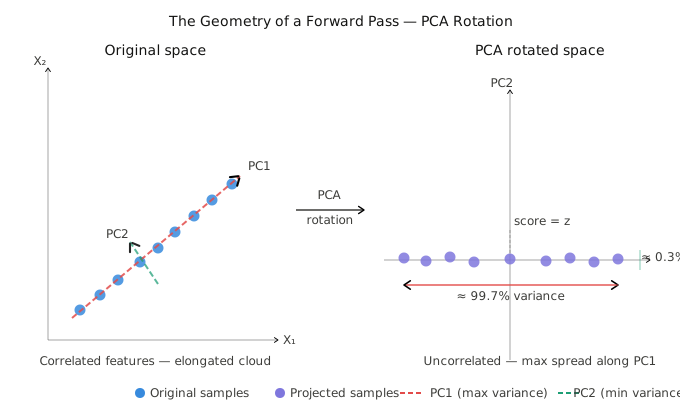
PCA rotates the coordinate system so that:
The first axis (PC1) points in the direction of greatest spread (maximum variance)
The second axis (PC2) is perpendicular to PC1 and captures the next greatest spread
And so on...
The loading vectors
v
i
\mathbf{v}_i
v i scores
Z
Z
Z
Explained Variance
Scree Plot
A scree plot shows eigenvalues in descending order. The "elbow" point suggests the optimal number of components.
Scree Rule: Choose components before the plot "levels off" (the elbow). In both examples, the elbow is clearly at PC1 , with all remaining components nearly flat.
(See PCA_Charts.html for interactive Scree Plots and PC1 Score charts for both examples.)
Choosing the Number of Components
Method 1: Cumulative Explained Variance (95% Rule)
k
∗
=
min
{
k
:
∑
i
=
1
k
λ
i
∑
j
=
1
p
λ
j
≥
0.95
}
k^* = \min\left\{ k : \frac{\sum_{i=1}^{k} \lambda_i}{\sum_{j=1}^{p} \lambda_j} \geq 0.95 \right\}
k ∗ = min { k : ∑ j = 1 p λ j ∑ i = 1 k λ i ≥ 0.95 } Method 2: Kaiser's Rule
Keep all components with eigenvalue
≥
1
\geq 1
≥ 1
k
∗
=
∣
{
i
:
λ
i
≥
1
}
∣
k^* = |\{i : \lambda_i \geq 1\}|
k ∗ = ∣ { i : λ i ≥ 1 } ∣ Method 3: Broken Stick Model
Component
i
i
i
λ
i
>
1
p
∑
j
=
i
p
1
j
\lambda_i > \frac{1}{p} \sum_{j=i}^{p} \frac{1}{j}
λ i > p 1 j = i ∑ p j 1 Method 4: Cross-Validation
k
∗
=
arg
min
k
CV-Error
(
k
)
k^* = \arg\min_k \text{CV-Error}(k)
k ∗ = arg k min CV-Error ( k ) Limitations of PCA
Limitation
Description
Alternative
Linearity PCA only captures linear relationships
Kernel PCA, Autoencoders
Interpretability PCs are abstract combinations of features
Sparse PCA, ICA
Scale sensitivity Sensitive to feature scale
Always standardize first
Outlier sensitivity Outliers can dominate principal components
Robust PCA
Gaussian assumption Works best with normally distributed data
ICA for non-Gaussian
Information loss Discarded components lose some information
Choose
k
k
k
Formula
Expression
Standardization
z
i
j
=
x
i
j
−
x
ˉ
j
σ
j
z_{ij} = \dfrac{x_{ij} - \bar{x}_j}{\sigma_j}
z ij = σ j x ij − x ˉ j
Mean
x
ˉ
j
=
1
n
∑
i
=
1
n
x
i
j
\bar{x}_j = \dfrac{1}{n}\displaystyle\sum_{i=1}^n x_{ij}
x ˉ j = n 1 i = 1 ∑ n x ij
Variance
σ
j
2
=
1
n
−
1
∑
i
=
1
n
(
x
i
j
−
x
ˉ
j
)
2
\sigma_j^2 = \dfrac{1}{n-1}\displaystyle\sum_{i=1}^n (x_{ij}-\bar{x}_j)^2
σ j 2 = n − 1 1 i = 1 ∑ n ( x ij − x ˉ j ) 2
Covariance matrix
Σ
=
1
n
−
1
X
′
T
X
′
\Sigma = \dfrac{1}{n-1} X'^T X'
Σ = n − 1 1 X ′ T X ′
Characteristic equation
det
(
Σ
−
λ
I
)
=
0
\det(\Sigma - \lambda I) = 0
det ( Σ − λ I ) = 0
Eigenvector equation
Σ
v
=
λ
v
\Sigma \mathbf{v} = \lambda \mathbf{v}
Σ v = λ v
Projection
Z
=
X
′
W
k
Z = X' W_k
Z = X ′ W k
Reconstruction
X
^
=
Z
W
k
T
+
X
ˉ
\hat{X} = Z W_k^T + \bar{X}
X ^ = Z W k T + X ˉ
Explained variance ratio
EVR
i
=
λ
i
∑
j
λ
j
\text{EVR}_i = \dfrac{\lambda_i}{\sum_j \lambda_j}
EVR i = ∑ j λ j λ i
Reconstruction error
Err
=
∑
i
=
k
+
1
p
λ
i
\text{Err} = \displaystyle\sum_{i=k+1}^{p} \lambda_i
Err = i = k + 1 ∑ p λ i
Summary
DATA (n × p) │ ▼ STANDARDIZE (optional, recommended) │ ▼ CENTER: X' = X - mean(X) │ ▼ COVARIANCE: Σ = (1/n-1) X'ᵀX' │ ▼ EIGENDECOMPOSITION: Σv = λv │ ▼ SORT eigenpairs: λ₁ ≥ λ₂ ≥ ... ≥ λₚ │ ▼ SELECT top-k components: Wₖ = [v₁|v₂|...|vₖ] │ ▼ PROJECT: Z = X'·Wₖ (n × k) │ ▼ REDUCED DATA (n × k), k << p
Key Takeaways
PCA is a rotation , not a selection — it creates new features from combinations of old onesEigenvalues = variance of each principal componentEigenvectors = directions of maximum variance (principal axes)Always standardize when features have different unitsThe trace is preserved :
∑
λ
i
=
∑
σ
j
2
\sum \lambda_i = \sum \sigma_j^2
∑ λ i = ∑ σ j 2 Use the 95% rule as a starting point for selecting
k
k
k PCA is linear — for non-linear data, consider Kernel PCA or t-SNE