Vectorization in Neural Networks

Table of Contents

1. What is Vectorization?
2. When to Use Vectorization
3. Mathematical Foundations
4. General Rules and Key Formulas
5. Step-by-Step Algorithm
6. Numerical Example 1 — Basic Dot Product (Single Neuron)
7. Numerical Example 2 — Two-Layer Neural Network
8. Comparing the Two Examples
9. Geometric Intuition
10. Advantages of Vectorization
11. Limitations of Vectorization
12. Complete Formula Reference
13. Summary

What is Vectorization?

Vectorization is a technique where operations are performed on entire arrays (vectors or matrices) at once, replacing explicit loops with compact linear-algebra expressions that hardware can execute in parallel.

Vectorization finds the most efficient representation of a computation by expressing it as matrix and vector operations, retaining the same numerical result while dramatically reducing wall-clock time.

Core Idea

Given a dataset with $n$ observations and $p$ features, and a weight vector $\mathbf{w} \in \mathbb{R}^p$, the output $z$ can be computed as:

• Loop-based: iterate over each element $w_i x_i$ one at a time
• Vectorized: compute $z = \mathbf{w}^T \mathbf{x} + b$ as a single dot product

When to Use Vectorization

Mathematical Foundations

Vector Representation

A single input sample with $p$ features is a column vector:

Dot Product (Single Neuron, No Bias)

Affine Transformation (Single Neuron with Bias)

Matrix Form — One Layer, $m$ Neurons, $n$ Samples

Where:

• $W \in \mathbb{R}^{m \times p}$ — weight matrix ($m$ neurons, $p$ inputs each)
• $X \in \mathbb{R}^{p \times n}$ — input matrix ($p$ features, $n$ samples)
• $\mathbf{b} \in \mathbb{R}^m$ — bias vector
• $Z \in \mathbb{R}^{m \times n}$ — pre-activation output

Activation Function (Element-wise)

Common choices: $g(z) = \sigma(z) = \dfrac{1}{1+e^{-z}}$ (sigmoid), $\text{ReLU}(z) = \max(0,z)$, $\tanh(z)$

General Rules and Key Formulas

Rule 1: Loop-Based vs. Vectorized

Loop (scalar):

Vectorized:

General Rule: Any summation $\sum_i w_i x_i$ over features or samples can be replaced by a single matrix/vector product.

Rule 2: Layer-Wise Forward Pass Formula

Key dimension rules (always verify these):

where $n^{[l]}$ = number of neurons in layer $l$, $m$ = number of training samples.

Rule 3: Speed Rule

Rule of thumb: On modern hardware, a vectorized matrix multiply on GPU can be $10\times$–$1000\times$ faster than the equivalent Python loop, depending on matrix size.

Rule 4: Gradient (Backprop) Vectorization

All three backprop formulas are matrix products — no loops required.

Rule 5: Memory and Numerical Considerations

Step-by-Step Algorithm

Algorithm: Vectorized Forward Pass — L-Layer Neural Network
 
Input:  Input matrix X ∈ ℝ^(p×m), weights {W^[l], b^[l]} for l = 1…L
Output: Final activation A^[L] ∈ ℝ^(n^[L]×m)
 
Step 1: INITIALISE
        A^[0] = X         (shape: p × m)
 
Step 2: FOR EACH LAYER l = 1 to L:
 
    Step 2a: LINEAR STEP
             Z^[l] = W^[l] · A^[l-1] + b^[l]
             (broadcasting adds b^[l] to every column)
 
    Step 2b: ACTIVATION STEP
             A^[l] = g^[l]( Z^[l] )     (element-wise)
 
Step 3: OUTPUT
        Ŷ = A^[L]
 
Step 4: COMPUTE LOSS (e.g., cross-entropy for classification)
        L = -(1/m) Σ_j [ y_j log(ŷ_j) + (1-y_j) log(1-ŷ_j) ]
 
Step 5: BACKPROP (vectorized)
        For l = L down to 1:
            dZ^[l]   = dA^[l] ⊙ g'^[l](Z^[l])
            dW^[l]   = (1/m) dZ^[l] · (A^[l-1])^T
            db^[l]   = (1/m) sum(dZ^[l], axis=1, keepdims=True)
            dA^[l-1] = (W^[l])^T · dZ^[l]
 
Step 6: UPDATE WEIGHTS
        W^[l] ← W^[l] - α · dW^[l]
        b^[l] ← b^[l] - α · db^[l]

Numerical Example 1 — Basic Dot Product (Single Neuron)

Scope: $p = 3$ input features, $1$ neuron, $n = 1$ sample — reduce a weighted sum to a single scalar output.

Step 1 — Define Inputs

Step 2 — Loop-Based Computation

Step 3 — Vectorized Computation

👉 Same result — one line 🔥

Step 4 — Apply Activation Function

Using sigmoid $\sigma(z) = \dfrac{1}{1 + e^{-z}}$:

Final Result — Example 1

A single dot product replaced three multiplications and two additions executed in a loop — and the pattern scales to millions of features with zero code change.

Numerical Example 2 — Two-Layer Neural Network

Scope: $p = 2$ input features, Layer 1 has $m_1 = 2$ neurons (ReLU), Layer 2 has $m_2 = 1$ neuron (Sigmoid). $n = 3$ training samples.

Step 1 — Define Inputs and Parameters

Input matrix ($p \times n = 2 \times 3$):

Layer 1 ($m_1 \times p = 2 \times 2$):

Layer 2 ($m_2 \times m_1 = 1 \times 2$):

Step 2 — Layer 1: Linear Step

Step 3 — Layer 1: Activation (ReLU)

All values are positive, so ReLU makes no change here.

Step 4 — Layer 2: Linear Step

Step 5 — Layer 2: Activation (Sigmoid)

Final Result — Example 2

All three samples processed simultaneously in one matrix multiply per layer — no outer loop over samples required.

Comparing the Two Examples

Geometric Intuition

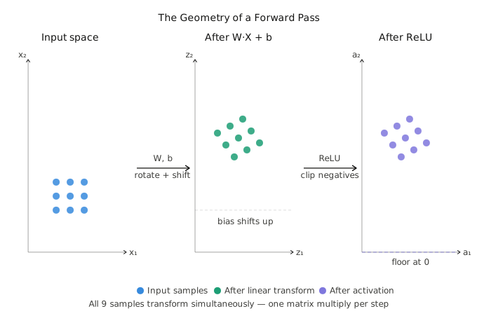
PCA rotates a coordinate system; vectorization transforms a dataset in the same spirit:

1. Weight matrix $W$ — applies a linear transformation (rotation + scaling) to the input space
2. Bias $b$ — shifts (translates) the transformed space
3. Activation $g$ — bends the space non-linearly

Instead of transforming one point at a time, the matrix multiply transforms all $n$ points simultaneously — this is the geometric essence of vectorization.

Advantages of Vectorization

Limitations of Vectorization

Complete Formula Reference

Summary

INPUT (p × m)
    │
    ▼
LAYER 1 — LINEAR:   Z¹ = W¹ · X + b¹
    │
    ▼
LAYER 1 — ACTIVATE: A¹ = g¹(Z¹)
    │
    ▼
LAYER 2 — LINEAR:   Z² = W² · A¹ + b²
    │
    ▼
LAYER 2 — ACTIVATE: A² = g²(Z²)
    │
    ▼
OUTPUT Ŷ = A^[L]   (all m samples processed at once)
    │
    ▼
LOSS → BACKPROP (all gradients are matrix products)
    │
    ▼
UPDATE WEIGHTS (W ← W − α · dW)

Key Takeaways

1. Vectorization = no loops — replace $\sum_i w_i x_i$ with $\mathbf{w}^T \mathbf{x}$
2. Batch processing — stack $m$ samples as columns; one matrix multiply handles all
3. Shape discipline — always verify $(m_l,\,m_{l-1}) \times (m_{l-1},\,n) = (m_l,\,n)$
4. Both forward and backward passes are fully vectorizable
5. Hardware wins — vectorized code automatically benefits from BLAS, CUDA, and TPU kernels
6. Same math, any scale — code for $n=3$ runs unchanged on $n=3{,}000{,}000$
7. Linear algebra is the language of deep learning — mastering it unlocks everything