Linear Discriminant Analysis (LDA)

Table of Contents

1. What is LDA?
2. LDA vs PCA
3. How LDA Works
4. LDA Mathematically
5. General Rules and Key Formulas
6. Step-by-Step Algorithm
7. Worked Example — From Lecture (6 Samples, 2 Features)
8. Worked Example — Quiz Problem (4 Samples, 2 Features)
9. Geometric Intuition
10. LDA as a Classifier
11. Limitations of LDA
12. Summary

What is LDA?

Linear Discriminant Analysis (LDA) is a supervised linear dimensionality reduction technique that finds the directions (called linear discriminants) maximizing the separation between multiple classes, while minimizing the spread within each class.

LDA finds the projection that maximizes between-class variance and minimizes within-class variance simultaneously.

Core Idea

Given a dataset with $n$ observations, $p$ features, and $C$ classes, LDA produces up to $C - 1$ new features (linear discriminants) that are:

• Class-aware — they use label information to guide the projection
• Ordered by the amount of class separation they provide
• Linear combinations of the original features

LDA vs PCA

Analogy: PCA finds the direction of greatest spread in the data. LDA finds the direction of greatest separation between classes.

How LDA Works

LDA seeks a projection direction $\mathbf{w}$ (a vector in the original feature space) such that, when data is projected onto it, the classes are as separated as possible.

The Two Objectives

1. Maximize between-class distance — the projected class means should be far apart.

2. Minimize within-class scatter — data points of the same class should cluster tightly around their projected mean.

Why Both Are Needed

Maximizing only the distance between means is insufficient — two classes can have well-separated means but heavily overlapping spreads, making classification unreliable. By also minimizing within-class scatter, LDA ensures a clean, non-overlapping separation.

LDA Mathematically

Projection

For a data point $\mathbf{x}$, its scalar projection onto direction $\mathbf{w}$ is:

where:

• $\mathbf{x} = [x_1, x_2, \ldots, x_p]^T$ is the original feature vector
• $\mathbf{w} = [w_1, w_2, \ldots, w_p]^T$ is the projection vector (analogous to PCA's eigenvector)
• $z$ is the scalar value after projection

Projected Means

For class $i$, the projected class mean is:

The overall projected mean is:

Between-Class Scatter Matrix $S_B$

The between-class variance measures how far apart the projected class means are from the overall projected mean:

Substituting $m_i = \mathbf{w}^T \boldsymbol{\mu}_i$ and $m_{\text{overall}} = \mathbf{w}^T \boldsymbol{\mu}_{\text{overall}}$, and using the matrix identity $(a^T b)^2 = a^T b b^T a$:

The term in parentheses is the between-class scatter matrix:

So: $\sigma_{\text{between}}^2 = \mathbf{w}^T S_B \mathbf{w}$

Within-Class Scatter Matrix $S_W$

The within-class variance for class $i$ measures how spread out the projected points are around their class mean:

Summing over all classes:

The term in parentheses is the within-class scatter matrix:

So: $\sigma_{\text{within}}^2 = \mathbf{w}^T S_W \mathbf{w}$

The Fisher Criterion and Eigenvalue Problem

The LDA objective becomes:

Maximizing $J(\mathbf{w})$ leads to the generalized eigenvalue problem:

Here, $\mathbf{w}$ is the eigenvector of $S_W^{-1} S_B$, and $\lambda$ is the eigenvalue. The eigenvector corresponding to the largest eigenvalue is the optimal projection direction LD1.

General Rules and Key Formulas

Rule 1: Class Mean Formula

Rule 2: Overall Mean Formula

Rule 3: Within-Class Scatter (compact form)

where $X_i$ is the submatrix of rows belonging to class $i$.

Rule 4: Between-Class Scatter

Rule 5: Eigenvalue Problem

Rule 6: Projection

Rule 7: Maximum Number of Discriminants

For $C$ classes, LDA produces at most $C - 1$ meaningful discriminant directions.

Step-by-Step Algorithm

Algorithm: Linear Discriminant Analysis (LDA)
 
Input:  Data matrix X ∈ ℝⁿˣᵖ with class labels, number of components k ≤ C-1
Output: Projected data Z ∈ ℝⁿˣᵏ, projection vectors W
 
Step 1: COMPUTE CLASS MEANS
        For each class i:  μᵢ = (1/nᵢ) Σ x  (for x in class i)
 
Step 2: COMPUTE OVERALL MEAN
        μ_overall = (1/n) Σ xⱼ  (over all samples)
 
Step 3: COMPUTE WITHIN-CLASS SCATTER MATRIX
        Sᵢ = (Xᵢ - μᵢ)ᵀ(Xᵢ - μᵢ)  for each class i
        S_W = Σ Sᵢ
 
Step 4: COMPUTE BETWEEN-CLASS SCATTER MATRIX
        S_B = Σ nᵢ(μᵢ - μ_overall)(μᵢ - μ_overall)ᵀ
 
Step 5: COMPUTE S_W⁻¹ S_B
 
Step 6: EIGENDECOMPOSITION
        Solve: det(S_W⁻¹S_B - λI) = 0  →  find λ₁ ≥ λ₂ ≥ ... ≥ λ_{C-1}
        For each λᵢ: solve (S_W⁻¹S_B - λᵢI)wᵢ = 0  →  find unit eigenvector wᵢ
 
Step 7: SELECT TOP-k DISCRIMINANTS
        W_k = [w₁ | w₂ | ... | wₖ]
 
Step 8: PROJECT DATA
        Z = X · W_k  ∈ ℝⁿˣᵏ

Worked Example — From Lecture (6 Samples, 2 Features)

Scope: $n = 6$ samples, $p = 2$ features, $C = 2$ classes → reduce to $k = 1$ discriminant (LD1).

Step 1 — Collect the Data

Step 2 — Compute Class Means

For Class 0 ($n_0 = 3$):

For Class 1 ($n_1 = 3$):

Step 3 — Compute Overall Mean

Step 4 — Compute Within-Class Scatter Matrix $S_W$

For Class 0 — center the class data:

For Class 1 — center the class data:

Total Within-Class Scatter:

Observation: $S_W$ is diagonal — features have no cross-class correlation within their respective classes.

Step 5 — Compute Between-Class Scatter Matrix $S_B$

For Class 0 ($n_0 = 3$):

For Class 1 ($n_1 = 3$):

Total Between-Class Scatter:

Step 6 — Compute $S_W^{-1} S_B$

Since $S_W = \begin{bmatrix} 4 & 0 \\ 0 & 4 \end{bmatrix}$ is diagonal:

Step 7 — Find Eigenvalues and Eigenvectors

Solve $\det(S_W^{-1} S_B - \lambda I) = 0$:

Find eigenvector for $\lambda_1 = 15.375$ (LD1):

Solve $(S_W^{-1} S_B - 15.375\,I)\mathbf{w} = \mathbf{0}$:

From row 1: $-6v_1 + 7.5v_2 = 0 \implies v_2 = \dfrac{6}{7.5} v_1 = 0.8\,v_1$

Setting $v_1 = 1$: $\mathbf{v} = [1,\ 0.8]^T$

Normalizing:

Interpretation: LD1 loads more heavily on $x_1$ than $x_2$, meaning $x_1$ contributes more to class separation.

Step 8 — Project the Data

Using $\mathbf{w} = [1, 0.8]^T$ (un-normalized, as in the lecture slides):

Final Result — Lecture Example:

Conclusion: Class 0 scores cluster in $[2.6,\ 4.4]$ and Class 1 scores cluster in $[10.0,\ 12.8]$ — a clean separation with no overlap on LD1!

Worked Example — Quiz Problem (4 Samples, 2 Features)

Source: Ahsanullah University of Science and Technology — CSE 4113, Pattern Recognition and Machine Learning, Quiz #03.
Problem: Reduce the dimension (from 2D to 1D) of the following dataset using Linear Discriminant Analysis.

Given Data

Two classes: Class 0 = {Sample 1, Sample 2}, Class 1 = {Sample 3, Sample 4}

Step 1 — Compute Class Means

For Class 0 ($n_0 = 2$, samples: $(1,2)$ and $(3,1)$):

For Class 1 ($n_1 = 2$, samples: $(6,5)$ and $(8,7)$):

Step 2 — Compute Overall Mean

Step 3 — Compute Within-Class Scatter Matrix $S_W$

For Class 0 — center the class data:

For Class 1 — center the class data:

Total Within-Class Scatter:

Step 4 — Compute Between-Class Scatter Matrix $S_B$

For Class 0 ($n_0 = 2$):

For Class 1 ($n_1 = 2$):

Total Between-Class Scatter:

Step 5 — Compute $S_W^{-1}$

For $S_W = \begin{bmatrix} 4 & 1 \\ 1 & 2.5 \end{bmatrix}$:

Step 6 — Compute $S_W^{-1} S_B$

Computing entry by entry:

Step 7 — Find Eigenvalues

Solve $\det(S_W^{-1} S_B - \lambda I) = 0$:

Note: $\lambda_2 \approx 0$ is expected — with 2 classes ($C = 2$), there is only 1 meaningful discriminant direction (maximum $C - 1 = 1$).

Step 8 — Find the Eigenvector for $\lambda_1 \approx 10.944$

Solve $(S_W^{-1} S_B - \lambda_1 I)\mathbf{w} = \mathbf{0}$:

From row 1: $-6.500\,v_1 + 4.000\,v_2 = 0 \implies v_2 = \dfrac{6.500}{4.000} v_1 = 1.625\,v_1$

Setting $v_1 = 1$: $\mathbf{v} = [1,\ 1.625]^T$

Normalizing:

Verification (row 2): $7.222(1) - 4.444(1.625) = 7.222 - 7.222 = 0$ ✅

Interpretation: LD1 loads more on $x_2$ than $x_1$ — feature $x_2$ contributes more to class separation in this dataset.

Step 9 — Project the Data

Using the un-normalized projection vector $\mathbf{w} = [1,\ 1.625]^T$:

Sample 1 (Class 0): $z_1 = 1(1) + 2(1.625) = 1 + 3.25 = 4.25$

Sample 2 (Class 0): $z_2 = 3(1) + 1(1.625) = 3 + 1.625 = 4.625$

Sample 3 (Class 1): $z_3 = 6(1) + 5(1.625) = 6 + 8.125 = 14.125$

Sample 4 (Class 1): $z_4 = 8(1) + 7(1.625) = 8 + 11.375 = 19.375$

Final Result — Quiz Problem:

Conclusion: Class 0 scores cluster in $[4.250,\ 4.625]$ and Class 1 scores cluster in $[14.125,\ 19.375]$ — near-perfect separation on a single dimension. The original 2D data is reduced to 1D while retaining maximum class discriminability!

Verification: Checking Class Separation

Projected Class Means:

Within-class variances (in LD1 space):

This matches our leading eigenvalue $\lambda_1 \approx 10.944$. ✅

The eigenvalue $\lambda_1$ is exactly the Fisher criterion value $J(\mathbf{w})$, confirming the solution is correct.

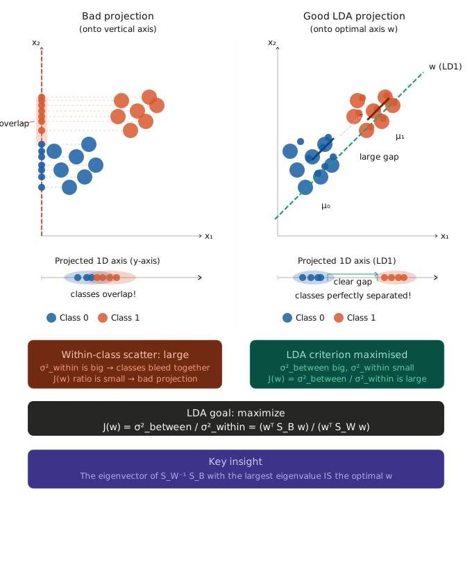
Geometric Intuition

LDA rotates and re-orients the coordinate system so that the new axis maximally separates the classes, rather than simply capturing the most variance (as PCA does).

The Projection Analogy

Think of projecting a 2D scatter plot down onto a 1D line — like shining a flashlight at the data and looking at the shadow. The question LDA answers is: what angle should the flashlight be at so the two class-shadows land as far apart as possible?

• Bad projection (left panel): Projecting onto the vertical axis ($x_2$) mixes the two classes together. Their projections heavily overlap — it is impossible to draw a clean boundary on this 1D line to separate them.

• Good LDA projection (right panel): The optimal direction $\mathbf{w}$ (LD1, green dashed line) is found by LDA. When data is projected perpendicularly onto this axis, Class 0 (blue) and Class 1 (coral) land in two compact, well-separated clusters with a clear gap between them.

What LDA Is Simultaneously Optimising

The green axis achieves two things at once:

1. Maximizes between-class scatter $S_B$ — the projected class means $m_0$ and $m_1$ are pushed as far apart as possible along $\mathbf{w}$.
2. Minimizes within-class scatter $S_W$ — each class's own points are pulled as tightly together as possible around their projected mean.

This simultaneous optimization is captured by the Fisher criterion:

The projection direction $\mathbf{w}$ that maximizes $J(\mathbf{w})$ is exactly the eigenvector of $S_W^{-1} S_B$ corresponding to its largest eigenvalue. The eigenvalue itself equals the maximum value of $J(\mathbf{w})$, confirming that LDA finds the theoretically optimal projection.

Summary: LDA does not merely pick the axis of greatest spread. It picks the axis that makes the class "shadows" as non-overlapping as possible — maximizing the gap between class means while minimizing the blur within each class.

LDA as a Classifier

Once the projection vector $\mathbf{w}$ is found, LDA can classify new data points.

Classification Steps

Step 1 — Project the new data point:

Step 2 — Compute projected class means:

Step 3 — Assign to the nearest class:

For 1D projection:

For multi-dimensional projections (multiple LDs):

Classifier Example (from lecture)

Using $\mathbf{w} = [1, 0.8]^T$ and a new point $\mathbf{x}_{\text{new}} = (5, 4)$:

Projected class means (from Step 8):

Distances:

Since $8.2$ is closer to $m_1 = 11.8$, the point is classified as Class 1. ✅

Limitations of LDA

Complete Formula Reference

Summary

DATA (n × p) with class labels
         │
         ▼
COMPUTE CLASS MEANS  μᵢ for each class i
         │
         ▼
COMPUTE OVERALL MEAN  μ_overall
         │
         ▼
WITHIN-CLASS SCATTER: S_W = Σᵢ (Xᵢ - μᵢ)ᵀ(Xᵢ - μᵢ)
         │
         ▼
BETWEEN-CLASS SCATTER: S_B = Σᵢ nᵢ(μᵢ - μ_overall)(μᵢ - μ_overall)ᵀ
         │
         ▼
COMPUTE  S_W⁻¹ S_B
         │
         ▼
EIGENDECOMPOSITION: S_W⁻¹ S_B w = λw
         │
         ▼
SORT eigenpairs: λ₁ ≥ λ₂ ≥ ... ≥ λ_{C-1}
         │
         ▼
SELECT top-k discriminants: W_k = [w₁ | w₂ | ... | wₖ]
         │
         ▼
PROJECT: Z = X · W_k  (n × k)
         │
         ▼
REDUCED DATA (n × k), maximally class-separable

Key Takeaways

1. LDA is supervised — it uses class labels to guide dimensionality reduction
2. Eigenvalue = Fisher criterion value — $\lambda_i = J(\mathbf{w}_i)$, the actual between/within ratio
3. Max $C - 1$ components — for binary classification, there is only ever 1 discriminant direction
4. $S_W$ must be invertible — if singular, use regularization or PCA pre-processing
5. LDA ≠ PCA — LDA maximizes class separation; PCA maximizes total variance and ignores labels
6. Classification by nearest projected mean — after projecting a new point onto LD1 (or LD space), assign it to the class whose projected mean is closest
7. Eigenvalue of $S_W^{-1} S_B$ — not of the covariance matrix; the matrix to decompose is $S_W^{-1} S_B$, not $\Sigma$